Spreadsheets: SPLCs as Stops
(North America only – SPLC data must be installed) To use SPLCs when entering origins/destinations, each number needs to be preceded by “ SPLC ”, e.g. “ SPLC191690000 ”. To add this text to a list of SPLCs in Microsoft® Excel, use the CONCATENATE formula as described below:
-
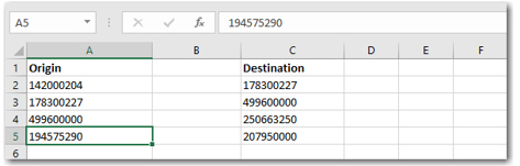
All origin SPLC numbers should be listed in one column (column A in this example). There should be at least one blank column to the right of the origins column.
-
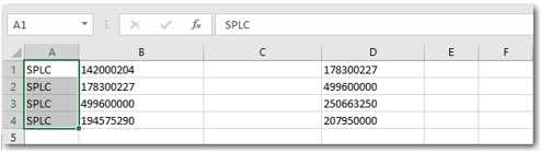
Insert a new column to the left of column A (right click column > Insert).
-
In the new column, add “SPLC” to each row that has a SPLC in it. To do this quickly, type “SPLC” in cell A1, then click and drag the bottom right corner of the cell down the column (the cursor will become a plus sign). Let go when all target cells are populated with “SPLC”.
-
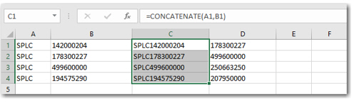
Select a third column to the right (column C in this example) and make sure the cells are formatted as “ General ” or “ Number ” (right click the column and choose Format Cells…).
-
In cell C1 (or C2 if there is a header row), manually enter the following formula: =CONCATENATE(A1,B1)
-
Copy the formula down the remainder of the column as in Step 3.
-
With the third column selected, right click and select Copy.
-
With the column still highlighted, right click and select Paste Special.
-
In the dialog that opens, select Values and hit OK.
-
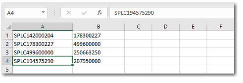
Delete the first two columns. Your origin SPLCs are now correctly formatted.
-
For the destination SPLC, follow steps 1-10 starting with the column that contain the destinations.
-
When you have origin and destination columns set up, you can enter a PC*Miler calculation function in the third column. Adjust the cell alignment and insert a header row if desired.
